Low R-squared values are not always bad and high R-squared values are not always good!

After you have fit a linear model using regression analysis, ANOVA (Analysis of variance), or design of experiments (DOE), you need to determine how well the model fits the data. [In this blog]https://blog.minitab.com/en/adventures-in-statistics-2/regression-analysis-how-do-i-interpret-r-squared-and-assess-the-goodness-of-fit), we’ll explore the R-squared (R2 ) statistic, some of its limitations, and uncover some surprises along the way. For instance, low R-squared values are not always bad and high R-squared values are not always good!

Table of Contents

What is Goodness-of-Fit for a linear model?

Linear regression calculates an equation that minimizes the distance between the fitted line and all of the data points. Technically, ordinary least squares (OLS) regression minimizes the sum of the squared residuals.

In general, a model fits the data well if the differences between the observed values and the model’s predicted values are small and unbiased.

Before you look at the statistical measures for goodness-of-fit, you should check the residual plots (Definition: Residual = Observed value - Fitted value). Residual plots can reveal unwanted residual patterns that indicate biased results more effectively than numbers. When your residual plots pass muster, you can trust your numerical results and check the goodness-of-fit statistics.

Roughly, Goodness-of-Fit indicates the discrepancy between observed values and the values expected under the model in question. ¹

What is R-squared?

R-squared is a statistical measure of how close the data are to the fitted regression line. It is also known as the coefficient of determination (可决系数), or the coefficient of multiple determination for multiple regression.

The definition of R-squared is fairly straight-forward; R-squared is the percentage of the response variable variation that is explained by a linear model. Or:

R-squared = Explained variation / Total variation
Measured with two sums of squares formulas:
$$ R^2 = 1-\frac{SS_{res}}{SS_{tot}} $$

The sum of squares of residuals, also called the residual sum of squares:

$$ SS_{res} = \sum_i (y_i-f_i)^2 = \sum_i e_i^2$$

The total sum of squares² (proportional to the variance of the data):

$$ SS_{tot} = \sum_i (y_i-\bar{y})^2$$

Note: $\bar {y}$ is the mean of the observed data.

R-squared is always between 0 and 100%:

• 0% indicates that the model explains none of the variability of the response data around its mean.
• 100% indicates that the model explains all the variability of the response data around its mean.
  
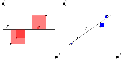
  $R^2 = 1- \frac{\color{blue}{SS_{res}}}{\color{red}{SS_{tot}}}$
  The better the linear regression (on the right) fits the data in comparison to the simple average (on the left graph), the closer the value of $R^2$ is to 1. The areas of the blue squares represent the squared residuals with respect to the linear regression. The areas of the red squares represent the squared residuals with respect to the average value.

In general, the higher the R-squared, the better the model fits your data. However, there are important conditions for this guideline that I’ll talk about both in this post and my next post.

Graphical representation of R-squared

Plotting fitted values by observed values graphically illustrates different R-squared values for regression models.

The regression model on the left accounts for 38.0% of the variance while the one on the right accounts for 87.4%. The more variance that is accounted for by the regression model the closer the data points will fall to the fitted regression line. Theoretically, if a model could explain 100% of the variance, the fitted values would always equal the observed values and, therefore, all the data points would fall on the fitted regression line.

Key limitations of R-squared

R-squared cannot determine whether the coefficient estimates and predictions are biased, which is why you must assess the residual plots.

R-squared does not indicate whether a regression model is adequate. You can have a low R-squared value for a good model, or a high R-squared value for a model that does not fit the data!

Are low R-squared values inherently bad?

No! There are two major reasons why it can be just fine to have low R-squared values.

In some fields, it is entirely expected that your R-squared values will be low. For example, any field that attempts to predict human behavior, such as psychology, typically has R-squared values lower than 50%. Humans are simply harder to predict than, say, physical processes.

Furthermore, if your R-squared value is low but you have statistically significant predictors, you can still draw important conclusions about how changes in the predictor values are associated with changes in the response value. Regardless of the R-squared, the significant coefficients still represent the mean change in the response for one unit of change in the predictor while holding other predictors in the model constant. Obviously, this type of information can be extremely valuable.

See a graphical illustration of why a low R-squared doesn’t affect the interpretation of significant variables.

A low R-squared is most problematic when you want to produce predictions that are reasonably precise (have a small enough prediction interval). How high should the R-squared be for prediction? Well, that depends on your requirements for the width of a prediction interval and how much variability is present in your data. While a high R-squared is required for precise predictions, it’s not sufficient by itself, as we shall see.

Are high R-squared values inherently good?

No! A high R-squared does not necessarily indicate that the model has a good fit. That might be a surprise, but look at the fitted line plot and residual plot below. The fitted line plot displays the relationship between semiconductor electron mobility and the natural log of the density for real experimental data.

The fitted line plot shows that these data follow a nice tight function and the R-squared is 98.5%, which sounds great. However, look closer to see how the regression line systematically over and under-predicts the data (bias) at different points along the curve. You can also see patterns in the Residuals versus Fits plot, rather than the randomness that you want to see. This indicates a bad fit, and serves as a reminder as to why you should always check the residual plots.

This example comes from my blog about choosing between linear and nonlinear regression. In this case, the answer is to use nonlinear regression because linear models are unable to fit the specific curve that these data follow.

However, similar biases can occur when your linear model is missing important predictors, polynomial terms, and interaction terms. Statisticians call this specification bias, and it is caused by an underspecified model. For this type of bias, you can fix the residuals by adding the proper terms to the model.

For more information about how a high R-squared is not always good a thing, read the blog Five Reasons Why Your R-squared Can Be Too High.